What four sample batches reveal about coarse particles and the value of SOP-based automated measurement

How closely do the particle size distributions of two silicon carbide abrasive batches match when both are made using the same process? And when the curves look similar overall, which local differences still deserve attention? A Bettersize application note examines four batches of black silicon carbide abrasive to show how the full distribution can help assess batch consistency. The A1 and A2 curves were broadly similar, but differences remained in the coarse region above 10 μm.

For abrasive manufacturers and quality control teams, this comparison helps pinpoint where batches differ. Reviewing the full curve alongside coarse- and fine-end metrics and repeat measurements helps identify the areas that need closer attention during quality assessment.

Read the full application note: Particle size distribution and quality inspection of four silicon carbide abrasive batches →

Why particle size distribution matters

Abrasive grains remove material through contact with the workpiece surface, so selecting a particle size involves balancing removal rate with surface finish. As the application note explains, finer grains generally remove material more slowly but help produce a smoother surface. Different machining tasks therefore call for different particle size distributions. For silicon carbide used in bonded abrasives, understanding the coarse, central and fine regions of a batch’s distribution helps connect material specifications with processing needs. This is why the study compares both batch distribution curves and several particle size metrics.

How the four batches were compared

The study used a Bettersizer ST laser particle size analyzer to measure four batches of black silicon carbide abrasive. A1 and A2 were produced using the same process parameters, with ISO/FEPA F1500 as the target grit designation. B1 and B2 also shared the same process parameters within their pair, with ISO/FEPA F320 as the target designation.

The study compares two pairs of production batches; it does not track one batch through successive processing steps. Read the curves as separate A1/A2 and B1/B2 comparisons, rather than as four repeat measurements of a single grit grade.

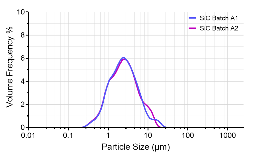
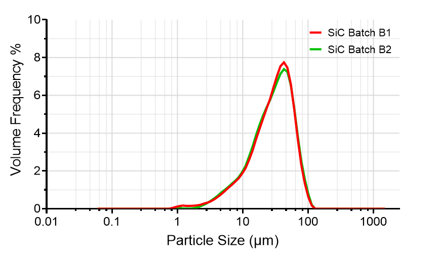
Particle size distributions for A1/A2 (top) and B1/B2 (bottom)

What to check when the curves look similar

Within each pair, the particle size distributions were broadly similar, although A1 and A2 differed in the coarse region above 10 μm. When sampling, dispersion and measurement conditions are consistent, curves with similar shapes and positions generally indicate good agreement between batch distributions. Repeat measurements, together with checks of the coarse, central and fine regions, provide a fuller basis for ongoing batch quality monitoring.

D50 describes the middle of the distribution. For a volume-based distribution, it is the particle diameter at which the cumulative volume fraction reaches 50%. It is not the maximum particle size, and it cannot describe the coarse and fine ends on its own.

Group A: Similar metrics, visible differences in the curves

Table 2 of the application note lists three particle size metrics for A1 and A2, along with comparison criteria from ISO 8486-2:2007, Bonded abrasives — Determination and designation of grain size distribution — Part 2: Microgrits F230 to F2000.

For this case, the notation follows ds(X) = D(100−X): ds3 = D97, ds50 = D50 and ds80 = D20. For example, ds3 (D97) is the diameter at which the cumulative volume fraction reaches 97%. In this volume-based distribution, approximately 97% of the total particle volume comes from particles smaller than that diameter.

A1 and A2 had similar D50 values of 2.256 μm and 2.294 μm, respectively, yet their curves still differed above 10 μm. A small set of characteristic particle sizes may therefore miss local changes in the distribution. Reading these values alongside the full curve makes such changes easier to spot and helps identify the particle size range in which they occur.

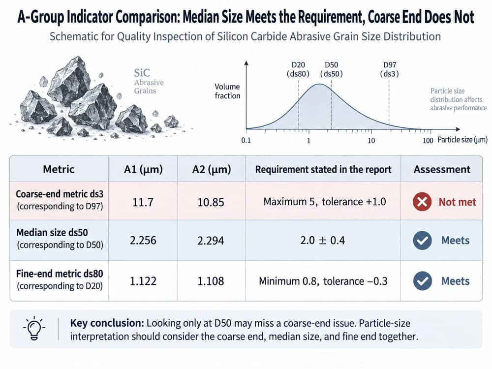
Group A metrics and the criteria cited in the application note. Both samples exceed the coarse-end requirement, despite their similar median sizes. Read characteristic values alongside the full distribution curve.

Group B highlights the need to check the fine end too

The B1/B2 comparison extends the discussion to both ends of the distribution. The application note considers coarse- and fine-end metrics together, showing why both belong in the same quality assessment. [1] In routine quality control, recording the coarse, central and fine regions helps teams spot shifts at different points in the distribution.

Batch curve comparisons and checks of individual metrics work well together. Curves reveal overall and local differences, while percentile diameters allow checks at specified points. Together, they provide a more complete picture than a single representative value.

Putting the case into practice in routine quality control

How can a particle size measurement guide the next step in quality improvement? Start with four questions: Are the samples comparable? Were the conditions consistent? Where do differences appear? What needs a closer look? The following four steps provide a practical way to read a report alongside your product specifications and production records.

How Bettersizer ST supports standardized testing with SOPs

For teams that test batches regularly, Bettersizer ST’s SOP-based automated measurement function organizes testing steps into a standardized workflow. Automatic alignment and wet dispersion form part of that workflow, helping operators follow preset steps and reducing the effort of repeatedly setting up and carrying out individual stages. [2] This makes repeat measurements and routine testing across batches easier to manage.

The application note reports 10–16 repeat measurements to examine the repeatability of sampling, dispersion and measurement. In routine quality control, teams can use Bettersizer ST’s SOP function to standardize repeat-testing workflows. It helps operators follow consistent measurement steps, leaving more time to evaluate results and monitor batch quality.

Bettersizer ST also combines wet dispersion and particle size analysis in a compact instrument, making it practical for routine testing in factories and laboratories. If you are developing a daily SOP for silicon carbide abrasive testing, bring your samples, target grit designation and quality requirements to a Bettersize application engineer. Together, you can discuss dispersion conditions, measurement steps and reporting metrics to develop a procedure suited to your samples.

Frequently asked questions

Is D50 enough to assess silicon carbide abrasive quality?

D50 summarizes the middle of a particle size distribution, but it may not capture local changes. For example, A1 and A2 had D50 values of 2.256 μm and 2.294 μm, yet their curves differed above 10 μm. Both contained too many large particles according to the criteria cited in the application note. A reliable assessment should consider repeat measurements, the full distribution curve and the relevant particle size metrics together.

What do similar particle size distribution curves tell us?

When sampling, dispersion and measurement conditions are consistent, curves with similar shapes and positions generally indicate good agreement between the two batch distributions. Comparing batches and their repeat measurements over time helps teams track changes and identify shifts at the coarse or fine end that need further investigation.

Is a coarse-end metric the same as the maximum particle size?

A coarse-end percentile diameter describes a specified point toward the larger-particle end of the distribution, not the maximum size. In this case, ds3 = D97: approximately 97% of the total particle volume comes from particles smaller than that diameter, with around 3% above it. Read coarse-end metrics alongside the curve rather than treating them as the size of the largest particle.

Why does the fine end need to be controlled?

The fine end describes the smaller-particle portion of the distribution. Along with the coarse end, it adds information that a central size value cannot provide. Tracking all three regions makes it easier to understand a batch’s distribution and see where differences emerge between batches.

What did Bettersizer ST measure in this study?

Bettersizer ST measured the particle size distributions of four batches of black silicon carbide abrasive for bonded abrasives, producing curves and size metrics for the A1/A2 and B1/B2 pairs. The distributions were broadly similar within each pair, while the A1/A2 curves revealed differences above 10 μm that warranted closer batch comparison.

How do I start developing a particle size testing procedure for silicon carbide abrasives?

First, define your sample type, target grit designation and the quality metrics you need to assess. Then discuss sampling, wet dispersion and repeat measurements with an application engineer. Bettersizer ST supports SOP-based automated measurement to help standardize routine testing. Including both the full curve and key metrics in your reports makes ongoing batch comparisons easier.