
- ● Introduction
- ● Nanoparticle Size and Zeta Potential Analyzer
- ● Theoretical background
- ● Optical Setup
- ● Monodisperse vs Polydisperse
- ● Data Interpretation
- ● Reference
- ● Backscattering Detection Technology
Introduction
Dynamic light scattering (DLS), also known as photon correlation spectroscopy (PCS), is a commonly used characterization method for nanoparticles. The DLS particle size analyzer has the advantages of accuracy, rapidity, and good repeatability for the measurement of nanoparticles, emulsions, or suspensions. The BeNano 180 Zeta Max nanoparticle analyzer is based on dynamic light scattering. It can measure nanomaterial down to 0.3 nanometers, which is an essential tool for nanoparticle size distribution measurement to understand and research nano-powdered materials.
Nanoparticle Size and Zeta Potential Analyzer
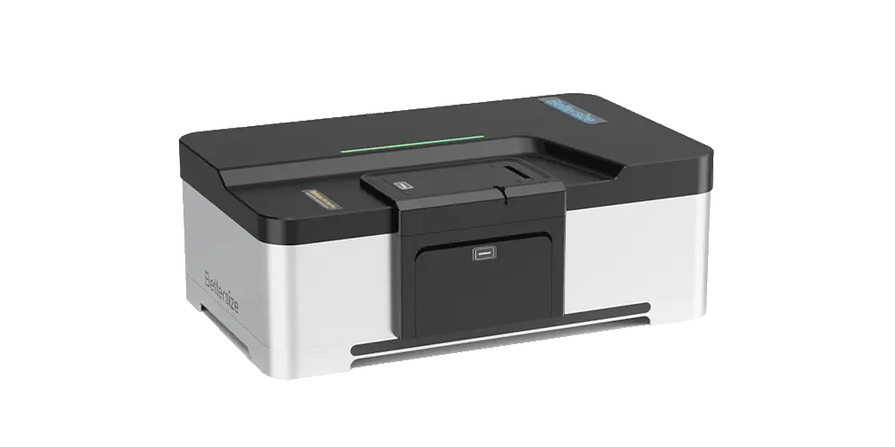
BeNano 180 Zeta Max
Nanoparticle Size and Zeta Potential Analyzer
Particle size measurement via sedimentation technology
Refractive index measurement
Particle concentration measurement
Theoretical Background
What is light scattering? When a monochromatic and coherent light source irradiates the particle, the electromagnetic wave will interact with the charges in atoms that compose the particle, and thus induce the formation of an oscillating dipole in the particle. Light scattering refers to the emission of light in all directions from an oscillating dipole. During quasi-elastic light scattering, the frequency changes between scattered light and incident light are small, and the light scattered by the oscillating dipole has a spectrum that broadens around the incident light frequency.
The scattered light intensity depends on the particle's intrinsic physical properties such as size and molecular weight. The scattered light intensity is not a constant value; it fluctuates over time due to the random walk of particles that are undergoing Brownian motion which refers to the particle's continuous and spontaneous random walk when placed in the medium resulting from the collisions between the particles and the medium molecules. The fluctuations in scattered light intensity with time allow us to calculate the diffusion coefficient through the auto-correlation function analysis. To quantify the speed of Brownian motion, the translational diffusion coefficient is modeled by the Stokes-Einstein equation. Notice here the diffusion coefficient is specified by the word “translational”, indicating that only the translational, but not the rotational movement of the particle is taken into account. The translational diffusion coefficient has the unit of area per unit of time, where the area is introduced to prevent the sign change convention when the particle is moving away from its origin. Then using the Stokes–Einstein equation, the particle size distribution can be calculated from the diffusion coefficient. This technique is called dynamic light scattering, abbreviated as DLS.
The Stokes-Einstein equation is expressed as follows:
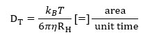
Equation 1: The Stokes-Einstein equation
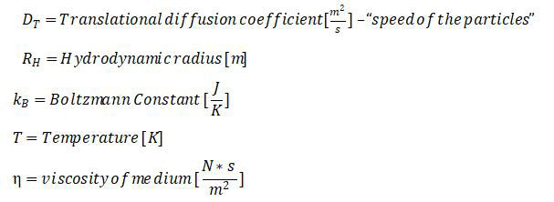
Hydrodynamic radius refers to the effective radius of a particle that has identical diffusion to a perfectly spherical particle of that radius. For example, as seen in figure 1, the true radius of the particle refers to the distance between its center and its outer circumference, while the hydrodynamic radius includes the length of the attached segments since they diffuse as a whole. Hydrodynamic radius is inversely proportional to the translational diffusion coefficient.
Figure 1: Illustration of hydrodynamic radius.
Optical Setup
The whole setup of DLS instrument is shown in Figure 2.
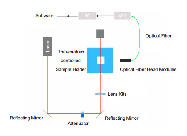
Figure 2: Dynamic light scattering optical set-up of BeNano 90, Bettersize Instruments.
- Laser
The majority of the laser devices in DLS instruments are gas lasers and solid-state lasers. Typical example of gas laser in DLS setup is helium-neon laser which emits laser with a wavelength of 632.8 nm. A solid-state laser refers to a laser device where a solid act as the gain medium. In a solid-state laser, small amounts of solid impurities called “dopant" are added to the gain medium to change its optical properties. These dopants are often rare-earth minerals such as neodymium, chromium, and ytterbium. The most commonly used solid-state laser is neodymium-doped yttrium aluminum garnet, abbreviated as Nd: YAG. Gas laser has the advantages of stable wavelength emission with relatively low cost. However, a gas laser usually has a relatively large volume that makes it very bulky. On the other hand, a solid-state laser is smaller in size and also less heavy, making it more flexible to handle.
- Detector
After the laser beam irradiates onto the sample cell, light is scattered by the particle, and this scattered light is fluctuated because of Brownian motion. A highly sensitive detector picks up these scattered light fluctuations signals at even low-intensity levels and converts them to electrical signals for further analysis in the correlator. Commonly used detectors in an optical setup of DLS include photomultiplier tube and avalanche photodiode. According to Lawrence W.G. et al., PMT and APD have similar noise to signal performance at most signal levels, while the APD outweighs the PMT at red and near-infrared spectral regions. APD also has higher absolute quantum efficiency than PMT. Because of these reasons, recently APD is being more frequently utilized in DLS devices.
- Correlator
After the optical setup, the process of scattering and collecting light intensity is completed. The signals detected by detectors are then analyzed in the correlator to eventually calculate the hydrodynamic radius distribution.
We can multiply the scattering intensity collected from the detector with itself after it has been shifted by some arbitrary interval tau (τ) in time. This τ can be anything between a few nanoseconds and microseconds, but the actual value of the time interval does not affect the test result.
After applying mathematical algorithm, the auto-correlation function G1(q, τ) can be obtained. G1(q, τ) single-exponentially decays from 1 to 0, with 0 meaning there's no correlation at all between signals at time t and time t plus τ, and 1 meaning perfect correlation. Finally, with all the known information of the correlation function, the hydrodynamic radius can be computed using the Stokes-Einstein equation.
Monodisperse vs. Polydisperse
Monodisperse particles are all identical in size, shape, and mass, resulting in one narrow peak in the particle size distribution curve. On the other hand, polydisperse particles are not uniform in those parameters. It is important to realize the polydispersity of the samples because the algorithms for calculating hydrodynamic radius distribution in the correlator are different depending on whether the samples are monodisperse or polydisperse.
Two main mathematical algorithms are used to solve the auto-correlation function of the polydisperse samples. The first and most common one is the Cumulants method, which involves solving the Taylor expansion of the auto-correlation function. However, the Cumulants method is only valid with samples that have small size polydispersity. Validation of the calculation can be done by computing and checking the polydispersity index, or PDI, and Cumulants analysis are only valid if the PDI value is relatively small. The CONTIN algorithm can directly compute the hydrodynamic radius distribution for samples that are widely dispersed. It is a relatively complicated mathematical method involving regularization.
Data Interpretation
Interpreting results can aid us in evaluating the quality of the particle size test, and also obtaining information about the particle size distribution.
The quality of the correlation function should be checked before proceeding to the particle size analysis since it directly relates to the accuracy of the particle size result. The overall shape of the correlation function could well indicate its quality. As shown in figure 6, if the correlation curve is a smooth curve exponentially decaying from 1 to 0 without the presence of noise, it suggests that the correlation was well performed and it is good to proceed to particle size distribution analysis.
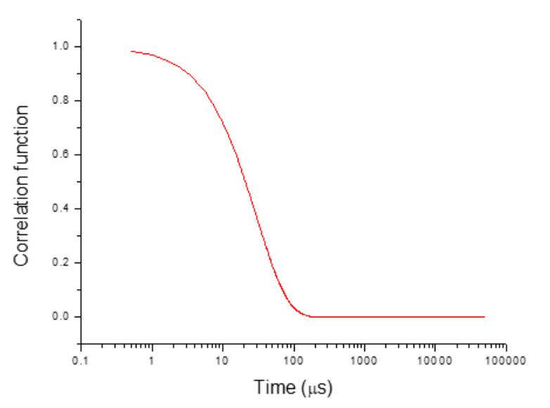
Figure 6: Example of a good correlation function curve.
However, if the curve is still overall smooth with some level of noise, as shown in figure 7, it might be due to the presence of impurities in the samples that affect the repeatability of the results. Under this scenario, the operator can filter the sample solution with the appropriate syringe pore size again to remove the impurities such as big dust particles in the solution.
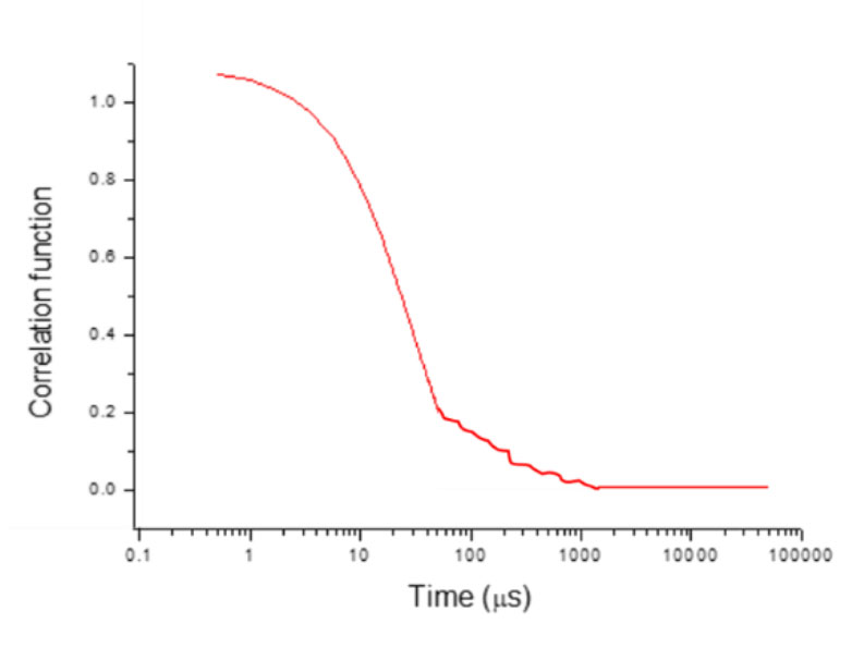
Figure 7: Example of a correlation function curve with noise.
When the scattering is insufficient in a test, its correlation function curve would look like the curve in figure 8.
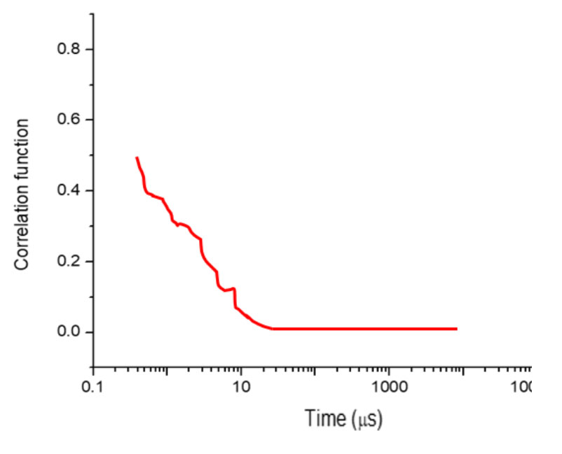
Figure 8: Example of a poor correlation function curve.
In this case, the maximum value of the function is much less than 1, and it does not exhibit exponential decay behavior. The operator could increase the sample concentration or the number of sub-runs to increase the amount of scattering.
DLS reports results in z-average particle size, which is a scattered intensity weighted size. It comes from the fact that when computing the correlation function integral using the Cumulants and CONTIN method, an average translational diffusion coefficient is obtained and thus resulting in the average hydrodynamic radius from the Stokes-Einstein equation. The z-average particle size’s validity should be checked with the polydispersity index or PDI. As shown in the table, a sample results report of particle size from DLS includes its z-average particle size with uncertainty, and the PDI value corresponding to that z-avg particle size.
If the value of PDI is large, indicating that the samples are possibly polydisperse, then the z-average particle size is not a fully representative description of the given sample.
According to the ISO 22412:2017 Particle Size analysis of dynamic light scattering, the particle size results should be reported along with its uncertainties and repeatability. The measurement uncertainty is expressed by the standard deviation, while the repeatability is the relative standard deviation that describes how close the results obtained from multiple measurements are to each other within each run of the test. As regulated by ISO 22412:2017, monodisperse materials with diameters between 50nm and 200nm should have z-avg particle size with repeatability of less than 2%.
Reference
Chu, B. Laser Light Scattering: Basic Principles and Practice, 2nd ed.; Academic Press: Boston, 1991.
Dian, L.; Yu, E.; Chen, X.; Wen, X.; Zhang, Z.; Qin, L.; Wang, Q.; Li, G.; Wu, C. Enhancing Oral Bioavailability of Quercetin Using Novel Soluplus Polymeric Micelles. Nanoscale Res Lett 2014, 9 (1), 684. https://doi.org/10.1186/1556-276X-9-684.
Dhont, J. K. G. An Introduction to Dynamics of Colloids; Studies in interface science; Elsevier: Amsterdam, Netherlands ; New York, 1996.
Falke, S.; Betzel, C. Dynamic Light Scattering (DLS): Principles, Perspectives, Applications to Biological Samples. In Radiation in Bioanalysis; Pereira, A. S., Tavares, P., Limão-Vieira, P., Eds.; Bioanalysis; Springer International Publishing: Cham, 2019; Vol. 8, pp 173–193. https://doi.org/10.1007/978-3-030-28247-9_6.
ISO 22412:2017. Particle Size Analysis – Dynamic Light Scattering (DLS). International Organization for Standardization.
Lawrence, W. G., Varadi, G., Entine, G., Podniesinski, E., & Wallace, P. K. (2008). A comparison of avalanche photodiode and photomultiplier tube detectors for flow cytometry. Imaging, Manipulation, and Analysis of Biomolecules, Cells, and Tissues VI. doi:10.1117/12.758958
Light Scattering from Polymer Solutions and Nanoparticle Dispersions; Springer Laboratory; Springer Berlin Heidelberg: Berlin, Heidelberg, 2007. https://doi.org/10.1007/978-3-540-71951-9.
Nanoscale Informal Science Education Network, NISE Network, Scientific Image – Gold Nanoparticles. Retrieved from https://www.nisenet.org/catalog/scientific-image-gold-nanoparticles.
Nanoparticles Series, Silicon Nanoparticles Product Details, ACS Materials. Retrieved from: https://www.acsmaterial.com/silicon-nanoparticles.html
Optical Sensors, Photomultiplier Tube, Newport Corporation. Retrieved from: https://www.newport.com/f/photomultiplier-tubes?q=PMT
Optoelectronic Components, Avalanche Photodiodes (APD), Warsash Scientific. Retrieved from: http://www.warsash.com.au/products/optoelectronics/PHOTONIC-DETECTORS.php
Scotti, A.; Liu, W.; Hyatt, J. S.; Herman, E. S.; Choi, H. S.; Kim, J. W.; Lyon, L. A.; Gasser, U.; Fernandez-Nieves, A. The CONTIN Algorithm and Its Application to Determine the Size Distribution of Microgel Suspensions. The Journal of Chemical Physics 2015, 142 (23), 234905. https://doi.org/10.1063/1.4921686.
Backscattering Detection Technology
With Intelligent Search For the Optimal Detection Position
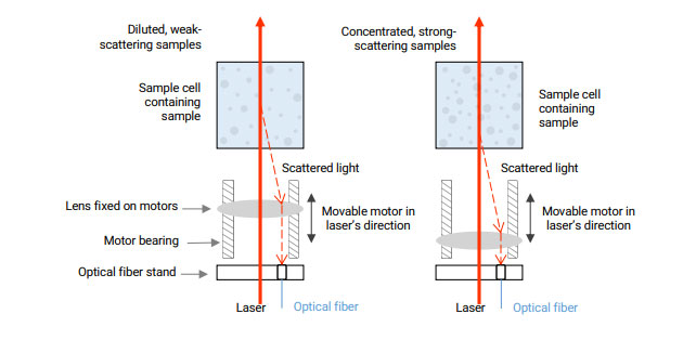
- The detection point is in the middle of the sample cell
As shown in the left graphic, the backscattering volume is so large that the detector receives many scattering signals from the particles and hence increases the sensitivity of the instrument. It has a better detection ability for dilute samples, which have smaller sizes and weaker scattering effects. However, the detection is not viable for samples with extremely high concentrations and very strong scattering effects. Even if the sample is barely detected, the result will deviate from the true value.
- The detection point is at the edge of the sample cell
As shown in the right graphic, the detection point is fixed near the wall of the sample cell. The laser beam does not need to penetrate the sample, which can effectively avoid the multiple scattering effect of high-concentration samples and ensure the accuracy and repeatability of the particle size results in the high concentration range. However, due to its optical design, the scattering volume is so small that impairs the sensitivity of the instrument, and hence the instrument is not competent to measure small particles, weak-scattering samples or very diluted samples under this condition
Solution: Intelligent search for the optimal detection position
By moving the lens, the detection point can be set at any position from the center to the edge of the sample cell. This allows the detection of different types and concentrations of samples to be considered to the extent possible. In practice, the optimal detection position and laser intensity are determined intelligently for each specific sample according to its sample concentration, size, and scattering ability in order to achieve the highest measurement accuracy.